The algorithm team at WSC Sports faced a challenge. How could our computer vision model, that is working in a dynamic environment, maintain high quality results? Especially as in our case, new data may appear daily and be visually different from the already trained data. Bit of a head-scratcher right? Well, we’ve developed a system that is doing just that and showing exceptional results!
But before introducing our model, or explaining the cause for extreme data changes that we face, let’s first understand our mission. At WSC Sports, we are using AI technologies to generate video highlights automatically from sports broadcasts, using action detection and event recognition algorithms. One of our main tasks is detecting replays and making sure they are linked to their corresponding event.
Replay recognition may look like an easy task, however, when observing an event, especially in sports broadcasts, our brain uses prior knowledge from years of experience. For example, when watching a sport broadcast on TV, we are able to distinguish between two different events that occurred at different times, and the same event being presented twice from different angles or at a different speed. Also, we can recognize special video editing patterns. In the case of replay events, they are usually surrounded by graphical overlays (figure1).

Figure 1 – example for slow motion replay followed by a graphic overlay
These kinds of recognition tasks require an understanding of broadcast conventions. As humans, we are able to understand broadcast patterns without the need to learn them explicitly. However, even for state-of-the-art machine learning tasks, it can be very challenging. To help us here, we developed a Replay Detection Model that learns broadcast patterns in sports to determine replay events.
As we mentioned earlier, a replay is an event that already happened and is shown again to the viewer from a different perspective (angle, speed, zoom, commentator comments, etc.). The Replay Detector Model aims to learn all these broadcast patterns in sport to determine replay events in videos.
The solution includes a convolutional neural network (CNN) backbone that aims to determine the optimal spatial features in each image, followed by a long short-term memory (LSTM) model that learns the temporal aspect of the video broadcasting (figure 2). Using the model outputs we are able to determine the replay action and its exact start and end times, resulting in a very accurate replay segment (figure 3).
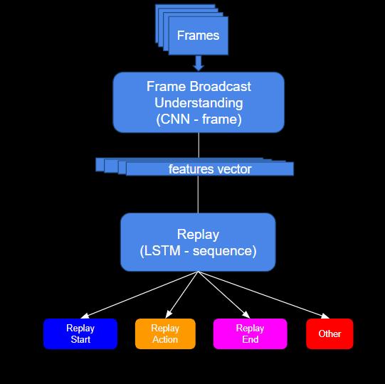
figure 2 – model architecture
figure 3 – results on football replay video clip
After deployment in production, the model worked surprisingly well, with very high performances.
However, WSC Sports is growing fast and we frequently sign new customers, so our model needs to handle frequent changes. With each new customer comes new data for a new sport, or extension of an existing sport, with new leagues and new variables to consider. Broadcast conventions can change rapidly from one sport to another and obviously from leagues, tournaments and across different countries. In some cases, the additional data is extremely different from what our model was used to process (new actions, backgrounds, broadcasting patterns, etc.).
Another cause for data changes comes from existing leagues that might change their broadcasting patterns between seasons. For example, some broadcasters may start using unusual graphics for the replay boundaries (figure 4) or don’t use graphics at all. Another example is drawings from pundits and commentators directly on the replay video, such as arrows or circles on players (figure 5). All these extreme data changes cause a drop in performance.
Suddenly, our initial model that got so many compliments, was just not good enough. We had to respond rapidly and retrain the model to support all the new sports and leagues. As we continued to grow the need to retrain the model became more frequent and required a lot of time-consuming effort: monitoring performances in production, tagging miss-detection, retraining the model, and testing its performance on all our sports and leagues.


figure 4 – unusual graphics for the replay boundaries

figure 5 – commentator drawing on video
To stay on top of all the new changes coming our way, and to maintain our high level of support and performance that our customers have come to expect, we had to find an automatic solution that would allow us to react quickly and efficiently to data drifts.
Pipeline Platform
Now that we understand the model architecture and outputs, we are ready to present the automatic pipeline solution we used for developing and improving models automatically.
We chose ClearML’s platform for developing the pipeline as it enables the easy creation of independent tasks on remote containers. For each task, we define its hierarchy in the process and the exact environment required for the task. Consequently, we can choose a different machine for each task and decrease the use of expensive resources (e.g GPU). In addition, we convert time-consuming tasks into multiple parallel tasks, which speed up the process exponentially.
The platform saves records of the inputs and outputs for each task. It also keeps track of the code’s version, data, and docker environment. All these abilities made the automatic process fast and feasible.
Pipeline Architecture
The pipeline consists of several main processes: data creation, training model, evaluation, deployment, and monitoring. Each process is triggered automatically when all the preceding steps in the hierarchy are complete (figure 6).
 figure 6 – pipeline process
Data Creation – this step includes obtaining videos that were misclassified in production, tagging these videos in a semi-automatic process and then cutting them into samples. Finally, uploading them to a dataset ready for training (train, test, validation). (figure 7).

figure 7 – data creation steps
We used queries that are responsible for retrieving new videos from our database for improving an existing sport. The database contains videos that are already categorized per sport and league. In addition, we have a record of incorrect predictions (reviewed manually) of our model results in production.
Then we use a basic Graphic Detection Model that is able to tag most of the sample’s graphics boundaries. The model has a very high recall for detecting graphic boundaries in videos, but it doesn’t have context; it cannot tell if a replay starts/ends or recognize any other temporal patterns mentioned earlier. However, we are using this simple model as a teacher within the context of a manual overview. It helps to cut video to samples representing: replay content, start, end and obviously, negative examples.
The automatic tagging phase ends with a set of videos ready to be cut and uploaded to a dataset. We also usually remain with a small portion of videos that get low confidence in the auto-tagging process and we send them to be manual review.
Training Model – this process includes training with different hyperparameters to achieve optimal performances on the test set. Using this pipeline helps us to explore a vast variety of experiments and more importantly helps to keep track of all the results and data versions. By performing tasks in parallel we were able to do more experiments and explore several hyperparameters and choose the optimal model.
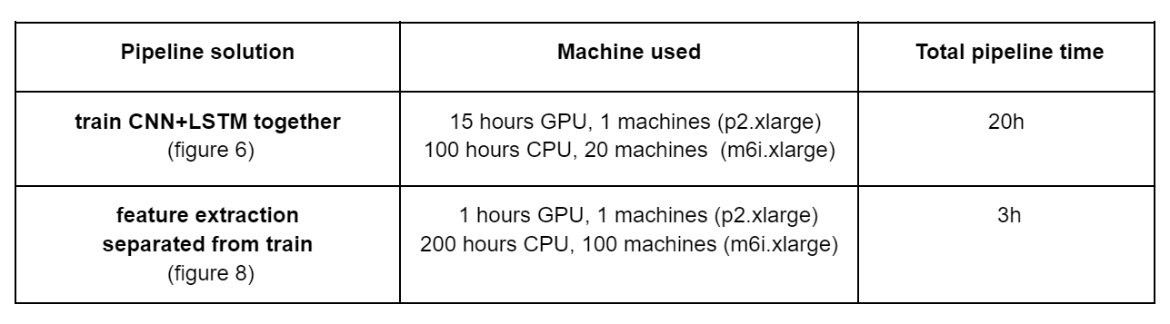
At first, training the model could take days. However, after training the model on a very large data set, we discovered that there is no need to train the backbone any more. We saw that the temporal features are the ones that frequently change and that in most cases training the temporal model, using the same spatial model, obtains very high performances. Using the trained CNN model only as a feature extractor (figure 8) was good enough and allowed us to use it as a preprocessing stage that can be executed in parallel. This made the training process much faster (from days to less than an hour). In addition, inference on the CNN alone didn’t require a machine with GPU and saved a lot of expenses.

figure 8 – pipeline process with feature extraction
To emphasize the impact of the separated feature extraction step, training the model on a new sport that includes 20,000 clips required 20 hours in the previous pipeline and now takes only 3 hours. Moreover, there was a significant decrease in the use of GPU machines.
Evaluation – the evaluation stage is executed with the same environment condition as production, using the optimal model. In this stage we use our validation set (or as we call it ‘golden set’), that is, a large set of videos that represent all the leagues and broadcasters of the sport we are focusing on.
At the end of this stage a detailed report is created and indicates the weakness of the league per sport and broadcaster signal (replay start, replay end, replay action signals, and the segment created from all the signals). For example, (Figure 8) we can see results of the evaluation process on basketball leagues after the automation process.
 Figure 8 – model results
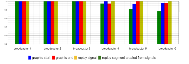
In this stage, we defined several tests to make sure we were able to improve the performance in terms of recall and precision for the problematic leagues and maintain the quality of the rest of the leagues.
Deployment & Monitoring – after successfully evaluating the results we then deploy our new model back to production. We monitor the model performances using conventional BI platforms. This step is disconnected from the automatic ClearML pipeline, but is necessary for triggering the continual learning process again when needed in the future.
Conclusion
After developing our continual learning pipeline, we were able to support rapid data changes in production. We disposed of unnecessary manual steps and parallelized every task possible (video tag, video cut, post logic) (Figure 9). The outcome means we can automate a process that previously took a few days, reducing the time to just a few hours!
Figure 9 – clearML pipeline ‘in action’. Each rectangle represents an individual task running on a machine. The colors represent the state of the task:
Light Blue: waiting to start, Green: in progress, Blue completed successfully, Red: failed.
What We Achieved Using the Pipeline
✅ Reduced development cycle significantly
✅ Spilt complicated tasks into sub-tasks
✅ Running tasks in parallel without worrying about manual errors